Machine Learning and phishing, pt. 1: Decision Trees

Table of Contents

Last week I started hunting and reporting phishing websites on Twitter (follow me here if you are interested). After some digging, I have decided that it would be interesting to use this topic to refresh my memory around the basics of Machine Learning.

In this series of posts I am going to use a smaller variant of this dataset to create machine learning models which (hopefully) will be able to identify a phishing website.

Please, note that the dataset contains the 10 ‘baseline features’ that were selected in this study.

The list of features and the code of this post in form of Jupyter notebook can be found here:

andpalmier/MLWithPhishing

Machine Learning basics with phishing dataset

Jupyter Notebook

This post has been inspired by:

A simple but effective decision tree

Let’s start with importing the libraries and the data. I used a csv version of the dataset, which you can find in the same GitHub repo linked above.

import numpy as np
from sklearn import tree

# Load the training data from a CSV file
training_data = np.genfromtxt('phishing_smaller.csv', delimiter=',', dtype=np.int32)

The csv has 10.000 samples with 11 columns, where the last one is the label of the sample, while the other values are the features.

# inputs are in all columns except the last one
inputs = training_data[:,:-1]

# outputs in the last column
outputs = training_data[:, -1]

We will use StratifiedKFold to keep the frequency of the classes constant during our K-fold cross-validation. The random_state parameter is used for k-fold and the classifier to reproduce the same setup for all the iterations of the model.

from sklearn.model_selection import StratifiedKFold

# use 10-fold
skf = StratifiedKFold(n_splits=10, random_state=0, shuffle=True)

In order to evaluate how good is our classifier, I will use AUC (Area Under Curve), you can find more information about it in this video:

Here is how to create, train and evaluate our first decision tree:

# library for evaluating the classifier
import sklearn.metrics as metrics

# array to store the accuracy during k-fold cross-validation
accuracy = np.array([])

# loop with splits
for train_index, test_index in skf.split(inputs, outputs):

    # 9 folds used for training
    X_train, X_test = inputs[train_index], inputs[test_index]
    # 1 fold for testing
    y_train, y_test = outputs[train_index], outputs[test_index]

    # Create a decision tree classifier
    classifier = tree.DecisionTreeClassifier(random_state=0)

    # Train the classifier
    classifier.fit(X_train, y_train)

    # Test the classifier
    predictions = classifier.predict(X_test)
    false_positive_rate, true_positive_rate, thresholds = \
        metrics.roc_curve(y_test, predictions)

    # calculate classifier accuracy
    ROC_AUC = metrics.auc(false_positive_rate, true_positive_rate)
    accuracy = np.append(accuracy,ROC_AUC)

print("ROC AUC: "+str(np.mean(accuracy)))

> ROC AUC: 0.9182929859719439

Not bad, but can we improve the accuracy of this decision tree with some tuning?

Tuning: criterion and splitter

If we take a look at the scikit-learn documentation for the decision tree classifiers, we can see that there are many parameters available. The first two are the criterion and splitter, having both two possible values. The supported criteria are gini (for Gini impurity) and entropy (for information gain); while the supported strategies available for splitting a node are best and random.

In total, we have 4 possible combinations: let’s try them to check which one performs better.

# AUC scores for test
results = []

# First= gini, best: default classifier
first_classifier = tree.DecisionTreeClassifier(random_state=0 \
    ,criterion="gini",splitter="best")

# Second= gini, random
second_classifier = tree.DecisionTreeClassifier(random_state=0 \
    ,criterion="gini",splitter="random")

# Third= entropy, best
third_classifier = tree.DecisionTreeClassifier(random_state=0 \
    ,criterion="entropy",splitter="best")

# Fourth= entropy, random
fourth_classifier = tree.DecisionTreeClassifier(random_state=0 \
    ,criterion="entropy",splitter="random")

# use same folds
StratifiedKFold(n_splits=10, random_state=0, shuffle=True)
for train_index, test_index in skf.split(inputs, outputs):

    X_train, X_test = inputs[train_index], inputs[test_index]
    y_train, y_test = outputs[train_index], outputs[test_index]

    # Train and test the first classifier
    first_classifier.fit(X_train, y_train)
    predictions = first_classifier.predict(X_test)
    false_positive_rate, true_positive_rate, thresholds = \
		metrics.roc_curve(y_test, predictions)
    # calculate classifier accuracy
    ROC_AUC = metrics.auc(false_positive_rate, true_positive_rate)
    first_accuracy = np.append(accuracy,ROC_AUC)

    # Train and test the second classifier
    second_classifier.fit(X_train, y_train)
    predictions = second_classifier.predict(X_test)
    false_positive_rate, true_positive_rate, thresholds = \
		metrics.roc_curve(y_test, predictions)
    # calculate classifier accuracy
    ROC_AUC = metrics.auc(false_positive_rate, true_positive_rate)
    second_accuracy= np.append(accuracy,ROC_AUC)

    # Train and test the third classifier
    third_classifier.fit(X_train, y_train)
    predictions = third_classifier.predict(X_test)
    false_positive_rate, true_positive_rate, thresholds = \
		metrics.roc_curve(y_test, predictions)
    # calculate classifier accuracy
    ROC_AUC = metrics.auc(false_positive_rate, true_positive_rate)
    third_accuracy= np.append(accuracy,ROC_AUC)

    # Train and test the fourth classifier
    fourth_classifier.fit(X_train, y_train)
    predictions = fourth_classifier.predict(X_test)
    false_positive_rate, true_positive_rate, thresholds = \
		metrics.roc_curve(y_test, predictions)
    # calculate classifier accuracy
    ROC_AUC = metrics.auc(false_positive_rate, true_positive_rate)
    fourth_accuracy= np.append(accuracy,ROC_AUC)

print("Test AUC for 'gini, best':       ",np.mean(first_accuracy))
print("Test AUC for 'gini, random':     ",np.mean(second_accuracy))
print("Test AUC for 'entropy, best':    ",np.mean(third_accuracy))
print("Test AUC for 'entropy, random':  ",np.mean(fourth_accuracy))

> Test AUC for 'gini, best':        0.9186236108580798
> Test AUC for 'gini, random':      0.9185325195846237
> Test AUC for 'entropy, best':     0.9184414283111678
> Test AUC for 'entropy, random':   0.9190781563126251

In this case, the fourth combination of criterion and splitter (criterion=entropy and split=random) seems to increase the performance of the classifier.

Tuning: max depth

Another parameter of the decision tree that we can tune is max_depth, which indicates the maximum depth of the tree. By default, this is is set to None, which means that nodes are expanded until all leaves are pure or contain less than min_sample_split samples.

Considering that we have 10 parameters, we will test the performances of trees having max_depths between 1 and 10.

# AUC scores for training and test
training_results = []
test_results = []

# use same folds
StratifiedKFold(n_splits=10, random_state=0, shuffle=True)

# from 1 to 10
max_depths = range(1,11)

for i in max_depths:

    # loop with splits
    for train_index, test_index in skf.split(inputs, outputs):
        training_accuracy = np.array([])
        test_accuracy = np.array([])

        X_train, X_test = inputs[train_index], inputs[test_index]
        y_train, y_test = outputs[train_index], outputs[test_index]

        # Create a decision tree classifier
        classifier = tree.DecisionTreeClassifier(random_state=0,max_depth=i)

        # Train the classifier
        classifier.fit(X_train, y_train)

        # Accuracy of the classifier during training
        training_predictions = classifier.predict(X_train)
        false_positive_rate, true_positive_rate, thresholds = \
            metrics.roc_curve(y_train, training_predictions)
        ROC_AUC = metrics.auc(false_positive_rate, true_positive_rate)
        training_accuracy = np.append(training_accuracy,ROC_AUC)

        # Test the classifier
        testing_predictions = classifier.predict(X_test)
        false_positive_rate, true_positive_rate, thresholds = \
            metrics.roc_curve(y_test, testing_predictions)

        # Accuracy of the classifier during test
        ROC_AUC = metrics.auc(false_positive_rate, true_positive_rate)
        test_accuracy = np.append(test_accuracy,ROC_AUC)

    # append results for line chart
    training_results.append(np.mean(training_accuracy))
    test_results.append(np.mean(test_accuracy))

In order to visualize the results, let’s use matplotlib to draw a line chart.

# training results in blue
line1, = plt.plot(max_depths, training_results, 'b', label='Train AUC')
# test results in red
line2, = plt.plot(max_depths, test_results, 'r', label='Test AUC')
plt.legend(handler_map={line1: HandlerLine2D(numpoints=2)})
plt.ylabel('AUC score')
plt.xlabel('Tree depth')
plt.show()

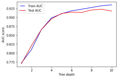
max depth chart — Performance of the model while tuning max_depth

As expected, increasing max_depth allows the model to be more specific when predicting the class of the given sample, thus improving the accuracy during training and test.

Tuning: min samples split

The next parameter is min_samples_split:

If int, it represents the minimum number of samples required to split an internal node.
If float, it is considered a fraction and ceil(min_samples_split * len(samples)) are the minimum number of samples for each split.

While the default value is 2, we will test the performance of our classifier having min_samples_split between 0.05 and 1.0.

# AUC scores for training and test
training_results = []
test_results = []

# use same folds
StratifiedKFold(n_splits=10, random_state=0, shuffle=True)

# from 5% to 100%
min_samples_splits = np.linspace(0.05, 1.0,20,endpoint=True)

for i in min_samples_splits:

    # loop with splits
    for train_index, test_index in skf.split(inputs, outputs):
        training_accuracy = np.array([])
        test_accuracy = np.array([])
        X_train, X_test = inputs[train_index], inputs[test_index]
        y_train, y_test = outputs[train_index], outputs[test_index]

        # Create a decision tree classifier
        classifier = tree.DecisionTreeClassifier(random_state=0,min_samples_split=i)

        # Train the classifier
        classifier.fit(X_train, y_train)

        # Accuracy of the classifier during training
        training_predictions = classifier.predict(X_train)
        false_positive_rate, true_positive_rate, thresholds = \
            metrics.roc_curve(y_train, training_predictions)
        ROC_AUC = metrics.auc(false_positive_rate, true_positive_rate)
        training_accuracy = np.append(training_accuracy,ROC_AUC)

        # Test the classifier
        testing_predictions = classifier.predict(X_test)
        false_positive_rate, true_positive_rate, thresholds = \
            metrics.roc_curve(y_test, testing_predictions)

        # Accuracy of the classifier during test
        ROC_AUC = metrics.auc(false_positive_rate, true_positive_rate)
        test_accuracy = np.append(test_accuracy,ROC_AUC)

    # append results for line chart
    training_results.append(np.mean(training_accuracy))
    test_results.append(np.mean(test_accuracy))

Let’s use another line chart to visualize the results:

# plot line chart
line1, = plt.plot(min_samples_splits, training_results, 'b', label='Train AUC')
line2, = plt.plot(min_samples_splits, test_results, 'r', label='Test AUC')
plt.legend(handler_map={line1: HandlerLine2D(numpoints=2)})
plt.ylabel('AUC score')
plt.xlabel('min samples split')
plt.show()

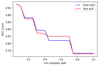
min samples split chart — Performance of the model while tuning min_samples_split

We can clearly see from the chart how increasing min_samples_split results in an underfitting case, where the model is not able to learn from the samples during training.

Tuning: min samples leaf

Similarly to the previous parameter, min_samples_leaf can be:

int, and it is used to specify the minimum number of samples required to be at a leaf node
if float, it represents a fraction and ceil(min_samples_leaf * n_samples) are the minimum number of samples for each node

By default, the value is set to 1, but we will consider the cases where it goes from 0.05 to 0.5.

# AUC scores for training and test
training_results = []
test_results = []

# from 5% to 50%
min_samples_leaves = np.linspace(0.05, 0.5, 10,endpoint=True)

for i in min_samples_leaves:

    StratifiedKFold(n_splits=10, random_state=0, shuffle=True)

    # loop with splits
    for train_index, test_index in skf.split(inputs, outputs):
        training_accuracy = np.array([])
        test_accuracy = np.array([])
        X_train, X_test = inputs[train_index], inputs[test_index]
        y_train, y_test = outputs[train_index], outputs[test_index]

        # Create a decision tree classifier
        classifier = tree.DecisionTreeClassifier(random_state=0, min_samples_leaf=i)

        # Train the classifier
        classifier.fit(X_train, y_train)

        # Accuracy of the classifier during training
        training_predictions = classifier.predict(X_train)
        false_positive_rate, true_positive_rate, thresholds = \
            metrics.roc_curve(y_train, training_predictions)
        ROC_AUC = metrics.auc(false_positive_rate, true_positive_rate)
        training_accuracy = np.append(training_accuracy,ROC_AUC)

        # Test the classifier
        testing_predictions = classifier.predict(X_test)
        false_positive_rate, true_positive_rate, thresholds = \
            metrics.roc_curve(y_test, testing_predictions)

        # Accuracy of the classifier during test
        ROC_AUC = metrics.auc(false_positive_rate, true_positive_rate)
        test_accuracy = np.append(test_accuracy,ROC_AUC)

    # append results for line chart
    training_results.append(np.mean(training_accuracy))
    test_results.append(np.mean(test_accuracy))

# plot line chart
line1, = plt.plot(min_samples_leaves, training_results, 'b', label='Train AUC')
line2, = plt.plot(min_samples_leaves, test_results, 'r', label='Test AUC')
plt.legend(handler_map={line1: HandlerLine2D(numpoints=2)})
plt.ylabel('AUC score')
plt.xlabel('min samples leaf')
plt.show()

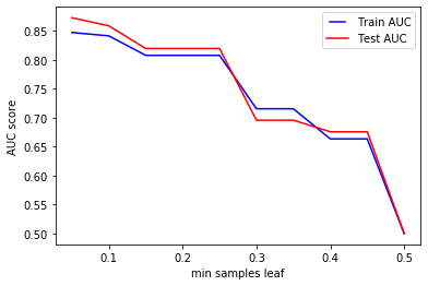
min samples leaf chart — Performance of the model while tuning min_samples_leaf

We can see that, similarly to the tuning of min_samples_split, increasing min_samples_leaf cause our model to underfit, drastically affecting the accuracy of the classifier during training and test.

Tuning: max features

The last parameter we are going to consider is max_features, which specifies the number of features to consider when looking for the best split.

If int, then consider max_features features at each split.
If float, is a fraction and int(max_features * n_features) features are considered at each split.
By default it is None, and max_features=n_features

Considering the number of features of our dataset, we will test measure the precision of classifiers having max_features between 1 and 10.

# AUC scores for training and test
training_results = []
test_results = []

# from 1 to 10 features
max_features = list(range(1,len(inputs[0])+1))

for i in max_features:

    StratifiedKFold(n_splits=10, random_state=0, shuffle=True)

    # loop with splits
    for train_index, test_index in skf.split(inputs, outputs):
        training_accuracy = np.array([])
        test_accuracy = np.array([])
        X_train, X_test = inputs[train_index], inputs[test_index]
        y_train, y_test = outputs[train_index], outputs[test_index]

        # Create a decision tree classifier
        classifier = tree.DecisionTreeClassifier(random_state=0,max_features=i)

        # Train the classifier
        classifier.fit(X_train, y_train)

        # Accuracy of the classifier during training
        training_predictions = classifier.predict(X_train)
        false_positive_rate, true_positive_rate, thresholds = \
            metrics.roc_curve(y_train, training_predictions)
        ROC_AUC = metrics.auc(false_positive_rate, true_positive_rate)
        training_accuracy = np.append(training_accuracy,ROC_AUC)

        # Accuracy of the classifier during test
        testing_predictions = classifier.predict(X_test)
        false_positive_rate, true_positive_rate, thresholds = \
            metrics.roc_curve(y_test, testing_predictions)

        # calculate classifier accuracy for test
        ROC_AUC = metrics.auc(false_positive_rate, true_positive_rate)
        test_accuracy = np.append(test_accuracy,ROC_AUC)

    # append results for line chart
    training_results.append(np.mean(training_accuracy))
    test_results.append(np.mean(test_accuracy))

# plot line chart
line1, = plt.plot(max_features, training_results, 'b', label='Train AUC')
line2, = plt.plot(max_features, test_results, 'r', label='Test AUC')
plt.legend(handler_map={line1: HandlerLine2D(numpoints=2)})
plt.ylabel('AUC score')
plt.xlabel('max features')
plt.show()

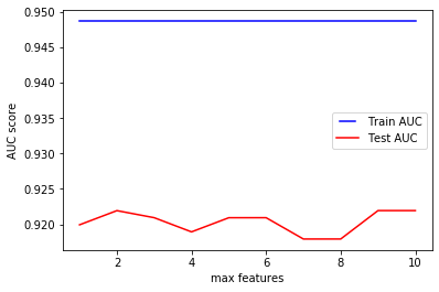
max features chart — Performance of the model while tuning max_features

We can see how the accuracy of the model does not seem to improve much when increasing the number of features considered during a split. While this may seem counter-intuitive, the scikit-learn documentation specifies that ‘the search for a split does not stop until at least one valid partition of the node samples is found, even if it requires to effectively inspect more than max_features features.’

Conclusion

These posts will investigate how tuning some of the available parameters can affect the performance of simple models. In this case, we saw how criterion, splitter, max_depth, min_samples_split, min_samples_leaf and max_features alter the predictions of a decision tree.

As pointed out from a friend, this is not the proper way of tuning the parameters of a model: one could extend parameters search by means of the RandomizedSearchCV provided by sklearn.