
I started hunting and reporting phishing pages on Twitter, follow me here if you are interested! After some digging, I have decided that it would be interesting to use this topic to refresh my memory around the basics of Machine Learning.
Introduction#
In the last post of this series, we analyzed how some of the parameters of a decision tree could improve the accuracy of the model when classifying phishing sites.

In this second post, we will perform a similar analysis, but with a different classifier: random forest.
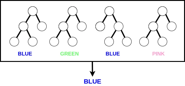
A random forest classifier is made of a number of decision trees which operate as an ensemble. The idea behind random forest is simple: every tree in the forest works independently as a classifier; then - based on the task which was submitted - the prediction of the forest is either the average of the predictions of the trees or the one with the most votes.
Random forest against phishing#
We will start the analysis by importing the libraries and the dataset which are going to be used in this post:
import numpy as np
from matplotlib.legend_handler import HandlerLine2D
from sklearn.ensemble import RandomForestClassifier
import matplotlib.pyplot as plt

# Load the data from a CSV file
train_data = np.genfromtxt('phishing_smaller.csv', delimiter=',', dtype=np.int32)
Our dataset contains 10.000 samples and 11 columns, where 10 represent the features and the last one is the label of the sample.
As for the previous episode, I used a smaller version of a dataset which was created for this study. You can find the version of the dataset used in this post here:
the repo contains also information about the features selected and the code of this post in form of a Jupyter notebook.
# inputs are in all columns except the last one
inputs = train_data[:,:-1]

# outputs in the last column
outputs = train_data[:, -1]
StratifiedKFold will be used in order to keep the frequency of the classes constant during our k-fold cross-validation. It is important to note that random_state is set not only for the k-fold validation, but also in the random forest classifier: this will ensure a reproducible setup for all iterations of the model.
from sklearn.model_selection import StratifiedKFold

# use 10-fold with random_state set to 0
skf = StratifiedKFold(n_splits=10, random_state=0, shuffle=True)
As in the other post, we will use AUC (Area Under Curve) to evaluate the accuracy of our classifier; so let’s import the required library and define the array to store the accuracy during the iterations with the different folds:
# library for evaluating the classifier
import sklearn.metrics as metrics

# list to store the accuracy during k-fold cross-validation
accuracy = np.array([])
We will now loop through the 10 splits and use them to train and evaluate 10 different models. The accuracy of these models will be stored in the accuracy list.
# loop with splits
for train_index, test_index in skf.split(inputs, outputs):

    # 9 folds used for training
    x_train, x_test = inputs[train_index], inputs[test_index]
    # 1 fold for testing
    y_train, y_test = outputs[train_index], outputs[test_index]

    # Creates the classifier
    # random_state is to keep same setup
    # n_jobs is -1 to use all the processors
    rf = RandomForestClassifier(random_state=0, n_jobs=-1)

    # Train the classifier
    rf.fit(x_train, y_train)

    # Test the classifier
    predictions = rf.predict(x_test)
    false_positives, true_positives, thresholds = \
        metrics.roc_curve(y_test, predictions)

    # calculate classifier accuracy
    ROC_AUC = metrics.auc(false_positives, true_positives)
    accuracy = np.append(accuracy,ROC_AUC)
The n_jobs parameter of the classifier defines the number of jobs to run in parallel over the trees. If set to None (which is the case by default) it means 1, while if set to -1 it will use all processors.
In order to evaluate our model trained with k-folds, we will take the mean of the accuracy of the 10 values generated in the previous steps:
print(f"ROC AUC: {np.mean(accuracy)}")> ROC AUC: 0.922092384769539The accuracy obtained is already quite good. In fact, it is better than the one obtained with the ‘vanilla’ decision tree. Let’s see which parameters could be used to improve the performance of our random forest.
Getting ready#
Before continuing with the analysis, considering that some actions are going to be repeated (training, testing and evaluate the classifiers) let’s wrap them in a function which will be called in the next paragraphs.
Our magic function will take in input a list of classifiers and two lists for the results of the training and testing. The lists for the results will be filled with the values of the AUC during the k-fold iterations and will be returned at the end of the function.
# function which takes as input a list of classifiers
# and two lists for the accuracy of the classifiers
# these 2 lists will be returned in the end
def magic(list_classifiers, list_train_accuracy, list_test_accuracy):

    # create the folds (always the same with random_state = 0)
    StratifiedKFold(n_splits=10, random_state=0, shuffle=True)
    for train_index, test_index in skf.split(inputs, outputs):

	x_train, x_test = inputs[train_index], inputs[test_index]
	y_train, y_test = outputs[train_index], outputs[test_index]

	# iterate through the classifiers
	for i in range(0,len(list_classifiers)):

	    classifier = list_classifiers[i]

	    classifier.fit(x_train, y_train)

	    # get train accuracy
	    predictions = classifier.predict(x_train)

	    false_positives, true_positives, threshold = \
		metrics.roc_curve(y_train,predictions)
	    ROC_AUC = metrics.auc(false_positives,true_positives)
	    list_train_accuracy[i] = np.append(list_train_accuracy[i],ROC_AUC)

	    # get test accuracy
	    predictions = classifier.predict(x_test)

	    false_positives, true_positives, threshold = \
		metrics.roc_curve(y_test,predictions)
	    ROC_AUC = metrics.auc(false_positives,true_positives)
	    list_test_accuracy[i] = np.append(list_test_accuracy[i],ROC_AUC)

    # return the array of accuracy of the classifiers
    return list_train_accuracy,list_test_accuracy
Choose the best criterion#
If you want to see the full list of parameters available to tune the random forest classifier, please refer to the scikit-learn documentation for random forest.
We will start our analysis with the criterion parameter, which represents the function that will be used to measure the quality of a split. The supported criteria are gini (for Gini impurity) and entropy (for information gain).
We will now create two classifiers having different criterion, to see which one has the best accuracy with our dataset.
# create the two classifiers
gini_classifier = RandomForestClassifier(random_state=0, \
    criterion="gini", n_jobs=-1)
entropy_classifier = RandomForestClassifier(random_state=0, \
    criterion="entropy", n_jobs=-1)

# lists to store variables to pass to the "magic" function
classifiers = [gini_classifier,entropy_classifier]
train_accuracies = [np.array([]),np.array([])]
test_accuracies = [np.array([]),np.array([])]

# in this iteration we are interested only in the test results
_,test_results = magic(classifiers,train_accuracies,test_accuracies)
print(f"Accuracy of gini classifier: {np.mean(test_results[0])}")
print(f"Accuracy of entropy classifier: {np.mean(test_results[1])}")

> Accuracy of gini classifier: 0.922092384769539
> Accuracy of entropy classifier: 0.9227925851703407
The results listed above shows that, even if the difference is not much (0.07%), the classifier using the entropy function as a criterion for the split outperforms the one using the gini function. It is interesting to note that the gini criterion is the one used by default for decision trees in sklearn.
Tuning: n_estimators#
Now we are going to tune n_estimators, which represents the total number of trees in the forest. Having a high number of trees usually has the advantage of increasing the overall accuracy of the model, however it will make the training phase slower due to the fact that a higher number of trees needs to be trained.
By default, n_estimators is set to 100 (before version 0.22 of sklearn it was 10).
In the following example, we will create and evaluate 8 different classifiers having n_estimators set to 1, 3, 6, 10, 25, 50, 75, 100, 125 and 150.
# number of estimators to use in the 10 classifiers
n_estimators = [1,3,6,10,25,50,75,100,125,150]

# lists to use for the "magic" function
classifiers = []
train_accuracies = []
test_accuracies = []

for i in n_estimators:

    # create classifier with appropriate n_estimators
    classifier = RandomForestClassifier(random_state=0, n_jobs=-1, n_estimators=i)
    classifiers.append(classifier)

    # metrics to evaluate the classifier
    train_accuracies.append(np.array([]))
    test_accuracies.append(np.array([]))

# let the magic happen
train_results,test_results = magic(classifiers,test_accuracies,train_accuracies)
The magic function returned two lists containing the accuracy for every iteration of k-fold for every classifier; now the average of the accuracy for each random forest will be taken, in order to show the results in a chart using matplotlib.
# store the averages of the classifiers for training and testing
avg_train=[]
avg_test=[]

# loop for every classifier we created
for i in range(0,len(train_results)):

    # average the results for every classifier
    avg_train.append(np.mean(train_results[i]))
    avg_test.append(np.mean(test_results[i]))

# blue line for train AUC
line1, = plt.plot(n_estimators, avg_train, 'b', label="Train AUC")
# red line for test AUC
line2, = plt.plot(n_estimators, avg_test, 'r', label="Test AUC")

# print chart
plt.legend(handler_map={line1: HandlerLine2D(numpoints=2)})
plt.ylabel('AUC score')
plt.xlabel('n_estimators')
plt.show()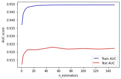
For our dataset, the best accuracy in the tests is achieved when using 50 trees (92,29%). If we further increase the number of trees, the AUC in the tests will slightly decrease. The same number of trees allows the classifier to reach the maximum accuracy during training (almost 95%).
Tuning: max_depth#
max_depth is used to specify the maximum depth of each tree in the forest. As we saw in our previous analysis, the deeper the tree, the more splits it has; thus it will be able to capure more information about the data.
The ranges of the max_depth for our analysis will be between 1 and 32. As in the previous paragraph, a line chart will be used to show the results.
# max depths to use in the classifiers
list_max_depth = np.linspace(1, 32, 32, endpoint=True)

# lists to use in the magic function
classifiers = []
train_accuracies = []
test_accuracies = []

for i in list_max_depth:

    # create classifier with appropriate max_depth
    classifier = RandomForestClassifier(random_state=0, n_jobs=-1, max_depth=i)
    classifiers.append(classifier)

    # metrics to evaluate the classifier
    train_accuracies.append(np.array([]))
    test_accuracies.append(np.array([]))

# let the magic happen
train_results,test_results = magic(classifiers,test_accuracies,train_accuracies)

# store the averages of the classifiers for training and testing
avg_training=[]
avg_testing=[]

for i in range(0,len(train_results)):

    # average the results for every classifier
    avg_training.append(np.mean(train_results[i]))
    avg_testing.append(np.mean(test_results[i]))

# blue line for train AUC
line1, = plt.plot(list_max_depth, avg_training, 'b', label="Train AUC")
# red line for test AUC
line2, = plt.plot(list_max_depth, avg_testing, 'r', label="Test AUC")

# print chart
plt.legend(handler_map={line1: HandlerLine2D(numpoints=2)})
plt.ylabel('AUC score')
plt.xlabel('max_depths')
plt.show()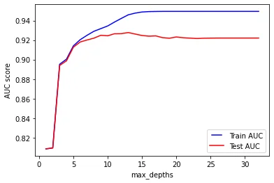
It is interesting to note the spike that is generated when increasing the max_depth of the trees in the forest from 2 to 3: the AUC in training and testing improves of almost 10% (from around 0.8 to almost 0.9).
As expected, max_depth contributes to an improvement of the overall accuracy of the model, until around 13, when the test AUC reach its peak. The best AUC during training is reached at 15, and remains stable even when using trees with 32 splits.
Tuning: min_samples_split#
The next parameter to be tuned is min_samples_split: it represents the minimum number of samples required to split a node in the trees of the forest. This parameter can be an integer (its default value is 2), but also a float: so that ceil(min_samples_split * n_samples) are the minimum number of samples for each split.
In this experiment will train and evaluate 10 classifiers having min_samples_split between 0.1 and 1.0.
# min samples splits from 10% to 100%
list_min_samples_splits = np.linspace(0.1,1.0,10,endpoint=True)

# lists to use in the magic function
classifiers = []
train_accuracies = []
test_accuracies = []

for i in list_min_samples_splits:

    # create classifier with appropriate max_depth
    classifier = RandomForestClassifier(random_state=0, n_jobs=-1, \
	min_samples_split=i)
    classifiers.append(classifier)

    # metrics to evaluate the classifier
    train_accuracies.append(np.array([]))
    test_accuracies.append(np.array([]))

# let the magic happen
train_results,test_results = magic(classifiers,test_accuracies,train_accuracies)

# store the averages of the classifiers for training and testing
avg_training=[]
avg_testing=[]

for i in range(0,len(train_results)):

    # average the results for every classifier
    avg_training.append(np.mean(train_results[i]))
    avg_testing.append(np.mean(test_results[i]))

# print chart
line1, = plt.plot(list_min_samples_splits, avg_training, 'b', label="Train AUC")
line2, = plt.plot(list_min_samples_splits, avg_testing, 'r', label="Test AUC")
plt.legend(handler_map={line1: HandlerLine2D(numpoints=2)})
plt.ylabel('AUC score')
plt.xlabel('min samples splits')
plt.show()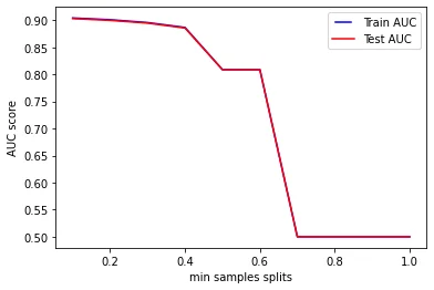
We can see from the results in the chart that for values of min_samples_split above 0.7, our model does not learn enough information from the data: this is because too many samples are required at each node in order to be split. For high values of min_samples_split the performances are equally bad (0.5 of AUC) during train and test.
Tuning: min_samples_leaf#
Similarly to the previous parameter, min_samples_leaf it is used to specify the minimum number of samples which are required to be in a leaf of the trees in our forest. Again, this parameter can be an integer (also in this case its default value is 2) and a float, so that ceil(min_samples_leaf * n_samples) are the minimum number of samples for each node.
The classifiers which are defined in the following lines have min_samples_split between 0.05 and 0.5 (maximum number allowed).
# min samples leaf from 5% to 50%
list_min_samples_leaf = np.linspace(0.05,0.5,10,endpoint=True)

# lists to use in the magic function
classifiers = []
train_accuracies = []
test_accuracies = []

for i in list_min_samples_leaf:

    # create classifier with appropriate max_depth
    classifier = RandomForestClassifier(random_state=0, n_jobs=-1, \
	min_samples_leaf=i)
    classifiers.append(classifier)

    # metrics to evaluate the classifier
    train_accuracies.append(np.array([]))
    test_accuracies.append(np.array([]))

# let the magic happen
train_results,test_results = magic(classifiers,test_accuracies,train_accuracies)

# store the averages of the classifiers for training and testing
avg_training=[]
avg_testing=[]

for i in range(0,len(train_results)):

    # average the results for every classifier
    avg_training.append(np.mean(train_results[i]))
    avg_testing.append(np.mean(test_results[i]))

# print chart
line1, = plt.plot(list_min_samples_leaf, avg_training, 'b', label="Train AUC")
line2, = plt.plot(list_min_samples_leaf, avg_testing, 'r', label="Test AUC")
plt.legend(handler_map={line1: HandlerLine2D(numpoints=2)})
plt.ylabel('AUC score')
plt.xlabel('min samples leaf')
plt.show()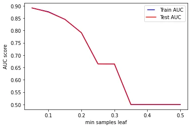
The results are similar to the previous analysis. Increasing the value of min_samples_leaf cause the model to fail in learning from the data, and decrease its performance to the point of obtaining AUC of 0.5 during train and test when min_samples_leaf is set to more than 0.35.
Tuning: max_features#
We will conclude this analysis of the random forest classifier with max_features. This parameter represents the number of features which are going to be considered when looking for the best possible split.
Its default value is None, so that max_features is set to the total number of features. Considering that our dataset has 10 features for every sample, we will train and test 10 classifiers having max_features between 1 and 10.
# max features from 1 to 10
list_max_features = range(1,11)

# lists to use in the magic function
classifiers = []
train_accuracies = []
test_accuracies = []

for i in list_max_features:

    # create classifier with appropriate max_depth
    classifier = RandomForestClassifier(random_state=0, n_jobs=-1, max_features=i)
    classifiers.append(classifier)

    # metrics to evaluate the classifier
    train_accuracies.append(np.array([]))
    test_accuracies.append(np.array([]))

# let the magic happen
train_results,test_results = magic(classifiers,test_accuracies,train_accuracies)

# store the averages of the classifiers for training and testing
avg_training=[]
avg_testing=[]

for i in range(0,len(train_results)):

    # average the results for every classifier
    avg_training.append(np.mean(train_results[i]))
    avg_testing.append(np.mean(test_results[i]))

# print chart
line1, = plt.plot(list_max_features, avg_training, 'b', label="Train AUC")
line2, = plt.plot(list_max_features, avg_testing, 'r', label="Test AUC")
plt.legend(handler_map={line1: HandlerLine2D(numpoints=2)})
plt.ylabel('AUC score')
plt.xlabel('max features')
plt.show()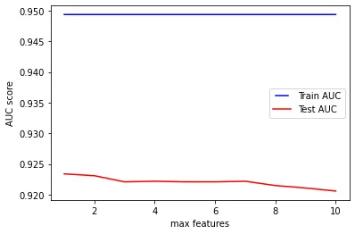
The resulting chart shows that the accuracy of the model does not improve when increasing max_features and it causes an overfitting for all the values in the experiment.
A similar result was obtained when tuning the same parameter for the decision tree. As stated in the sklearn documentation of random forest classifiers: ’the search for a split does not stop until at least one valid partition of the node samples is found, even if it requires to effectively inspect more than max_features features’.
Conclusion#
In this post we conducted an experiment to evaluate how some of the parameters available to tune random forest classifiers affect the performance of the model when trying to detect a phishing page. The parameters explored were: criterion, max_depth, min_samples_split, min_samples_leaf and max_features.
I will mention again that this is not the proper way of tuning the parameters for a random forest: the best approach would be to extend parameters search using RandomizedSearchCV provided by sklearn.